Regression Model Series II: Do Some Nonlinear Regression Models In R By Boston Housing Data Set
2016-02-29
This article continue to talk about regression model by Boston Housing data set.
Neural Networks
Neural networks is a strong nonlinear regression models made by ideas about how the brain works.
It is apt to over-fit the relationship between the predictors and the response, so we add penalty term like ridge regression called “weight decay” to combat this problem.
# load the data set
library(mlbench)
data(BostonHousing)

#########################
### split the data
#########################
library(caret)
set.seed(1234)
train_index <- createDataPartition(BostonHousing$medv, p = .8, list = FALSE)
trainset <- BostonHousing[train_index, ]
testset <- BostonHousing[-train_index, ]

###############################################
### nerual networks
# need preprocess to data

# since the regression coefficients are being summed
# they should be on the same scale
# the predictors should be centered and scaled prior to modeling

# since they use gradients to optimize the model parameters
# they are often adversly affected by high correlation
# pca can be used prior to modeling to eliminate correlations

nnet_grid <- expand.grid(decay = c(0, 0.01, .1),
                        size = c(1, 3, 5, 7, 9, 11, 13),
                        bag = FALSE)

set.seed(1234)
nnet_model <- train(medv ~ .,
                   data = trainset,
                   # similar nnet function in nnet package
                   method = "avNNet",
                   tuneGrid = nnet_grid,
                   trControl = trainControl(method= "cv"),
                   preProc = c("center", "scale"),
                   # linear relationship between the hidden units and the prediction
                   linout = TRUE,
                   # reduce the amount of printed output
                   trace = FALSE,
                   # the number of parameters used by the model
                   # 13 is the number of size (hidden units)
                   MaxNWts = 13 * ncol(trainset) + 13 + 1,
                   # the number of iterations to find parameter estimates
                   maxit = 1000,
                   allowParallel = FALSE)
nnet_model
## Model Averaged Neural Network
##
## 407 samples
## 13 predictor
##
## Pre-processing: centered (13), scaled (13)
## Resampling: Cross-Validated (10 fold)
## Summary of sample sizes: 366, 367, 365, 366, 366, 366, ...
## Resampling results across tuning parameters:
##
## decay size RMSE Rsquared MAE
## 0.00 1 4.275011 0.8061122 3.028067
## 0.00 3 3.617309 0.8570792 2.519298
## 0.00 5 3.890826 0.8318688 2.615542
## 0.00 7 3.569638 0.8616122 2.460702
## 0.00 9 3.643242 0.8570123 2.494616
## 0.00 11 3.431441 0.8731502 2.417719
## 0.00 13 3.607122 0.8559927 2.588893
## 0.01 1 4.239871 0.8019774 2.945607
## 0.01 3 3.334194 0.8713781 2.361733
## 0.01 5 3.423354 0.8743029 2.410203
## 0.01 7 3.557479 0.8615975 2.470570
## 0.01 9 3.515907 0.8647760 2.490476
## 0.01 11 3.439967 0.8726716 2.417719
## 0.01 13 3.195862 0.8896835 2.291567
## 0.10 1 4.275792 0.7986765 3.004531
## 0.10 3 3.442440 0.8705878 2.387252
## 0.10 5 3.510398 0.8678077 2.385664
## 0.10 7 3.575050 0.8621858 2.436488
## 0.10 9 3.306660 0.8806371 2.334304
## 0.10 11 3.166684 0.8940954 2.281979
## 0.10 13 3.269687 0.8876600 2.269570
##
## Tuning parameter 'bag' was held constant at a value of FALSE
## RMSE was used to select the optimal model using the smallest value.
## The final values used for the model were size = 11, decay = 0.1 and bag = FALSE.nnet_pred <- predict(nnet_model, testset)
postResample(pred = nnet_pred, obs = testset$medv)## RMSE Rsquared MAE
## 2.9408702 0.8627236 1.9893110# the plot of performance of model
df_nnet <- data.frame(predicted = nnet_pred, observed = testset$medv,
residual = testset$medv - nnet_pred)
ggplot(df_nnet, aes(x = predicted, y = observed)) +
geom_point() +
geom_abline(intercept = 0, slope = 1, colour = "blue") +
ggtitle("NNet Predicted VS Observed")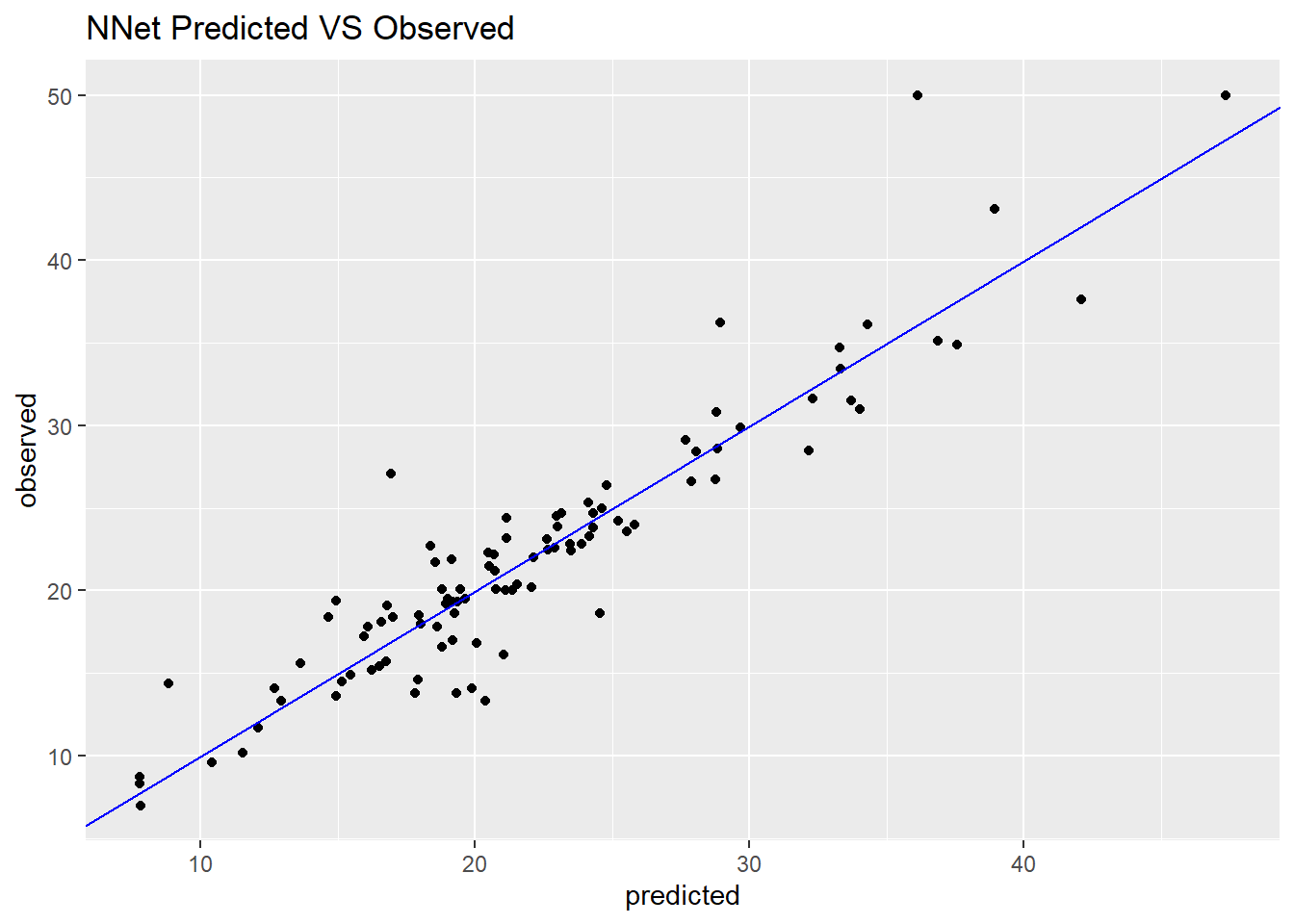
ggplot(df_nnet, aes(x = predicted, y = residual)) +
  geom_point() +
  geom_hline(yintercept = 0, colour = "blue") +
  ggtitle("NNet Predicted VS Residual")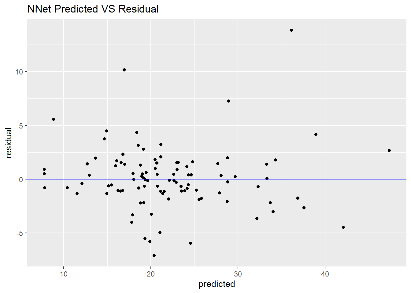
Although this performance of nonlinear model is better than our above linear model, the complex of neural network is much more than the simple linear regression.
The cross-validated RMSE profiles of neural network are displayed in below figure.
Increasing the number of weight decay clearly decrease RMSE and increase model stable.
When decay is 0.1, hidden units is 11, we get the optimal model.
plot(nnet_model)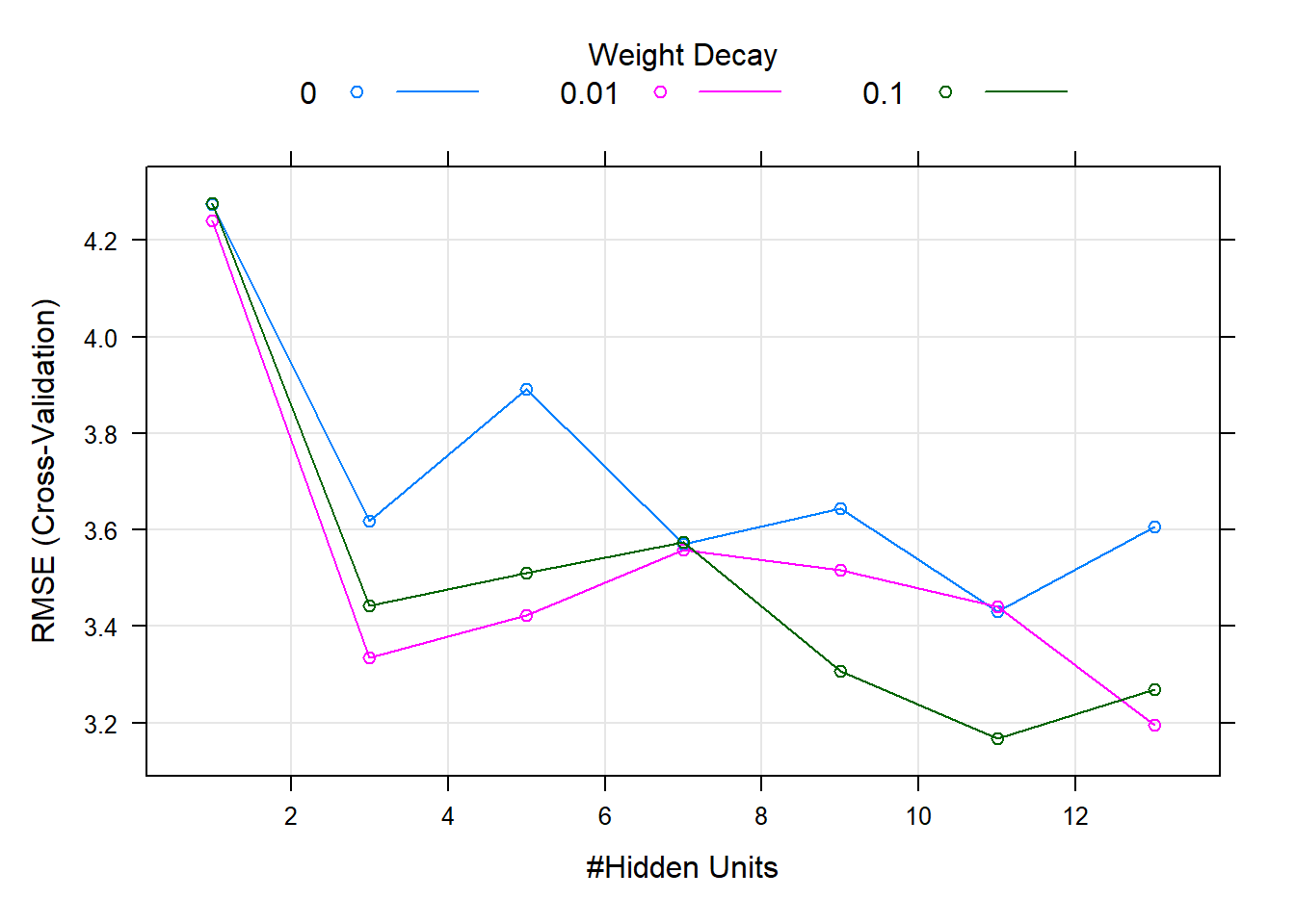
Multivariate Adaptive Regression Splines (MARS)
The nature of the MARS features breaks the predictor into two groups and models linear relationships between the predictor and the outcome in each group.
There are two tuning parameters with MARS model: the degree of the features and the number of terms.
MARS model conducts feature selection.
The cross-validation procedure picked a model with 19 nprune and was a function of 8 predictors.
From the figure of predicted VS observed and predicted VS residual, when the predicted of price of housing is above 35, the more far from the observed value.
The key predictors are average number of rooms per dwelling (rm), then percentage of lower status of the population (lstat), the third important ingredient is pupil-teacher ratio by town, then transport index (dis, rad), environment index (nox), tax rate, crime rate.
#####################################################
### multivariate adaptive regression splines (MARS)
set.seed(1234)
mars_model <- train(medv ~ .,
                   data = trainset,
                   method = "earth",
                   tuneGrid = expand.grid(degree = 1, nprune = 2:38),
                   trControl = trainControl(method= "cv"))
## 载入需要的程辑包:earth## 载入需要的程辑包:Formula## 载入需要的程辑包:plotmo## 载入需要的程辑包:plotrix## 载入需要的程辑包:TeachingDemosmars_model## Multivariate Adaptive Regression Spline
##
## 407 samples
## 13 predictor
##
## No pre-processing
## Resampling: Cross-Validated (10 fold)
## Summary of sample sizes: 366, 367, 365, 366, 366, 366, ...
## Resampling results across tuning parameters:
##
## nprune RMSE Rsquared MAE
## 2 6.287274 0.5855737 4.599592
## 3 4.685731 0.7695507 3.214606
## 4 4.329676 0.7984970 3.100716
## 5 4.242693 0.8066185 2.982543
## 6 4.278397 0.8054031 2.945634
## 7 4.090349 0.8220690 2.885269
## 8 4.001657 0.8279192 2.833056
## 9 3.707738 0.8509500 2.685786
## 10 3.680490 0.8541468 2.663916
## 11 3.674242 0.8547507 2.648238
## 12 3.629238 0.8601885 2.594235
## 13 3.659154 0.8577369 2.634606
## 14 3.637761 0.8600221 2.644861
## 15 3.675640 0.8591896 2.651940
## 16 3.668821 0.8598444 2.657905
## 17 3.709683 0.8563081 2.699340
## 18 3.702931 0.8580203 2.686478
## 19 3.692044 0.8592045 2.679226
## 20 3.692044 0.8592045 2.679226
## 21 3.692044 0.8592045 2.679226
## 22 3.692044 0.8592045 2.679226
## 23 3.692044 0.8592045 2.679226
## 24 3.692044 0.8592045 2.679226
## 25 3.692044 0.8592045 2.679226
## 26 3.692044 0.8592045 2.679226
## 27 3.692044 0.8592045 2.679226
## 28 3.692044 0.8592045 2.679226
## 29 3.692044 0.8592045 2.679226
## 30 3.692044 0.8592045 2.679226
## 31 3.692044 0.8592045 2.679226
## 32 3.692044 0.8592045 2.679226
## 33 3.692044 0.8592045 2.679226
## 34 3.692044 0.8592045 2.679226
## 35 3.692044 0.8592045 2.679226
## 36 3.692044 0.8592045 2.679226
## 37 3.692044 0.8592045 2.679226
## 38 3.692044 0.8592045 2.679226
##
## Tuning parameter 'degree' was held constant at a value of 1
## RMSE was used to select the optimal model using the smallest value.
## The final values used for the model were nprune = 12 and degree = 1.# mars_model$finalModel
# summary(mars_model$finalModel)
plot(mars_model)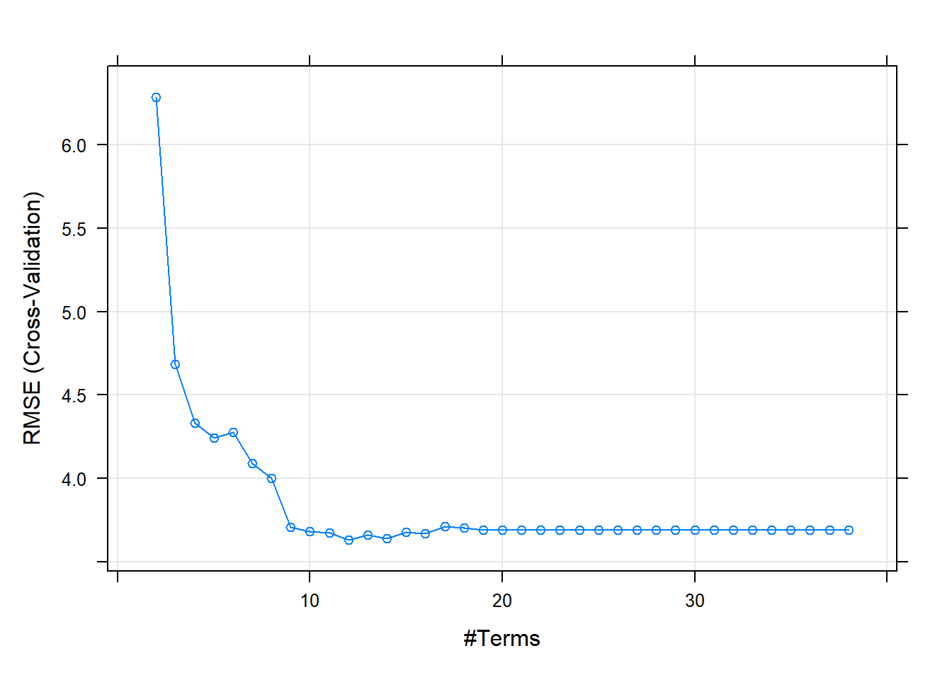
mars_pred <- predict(mars_model, testset)
postResample(pred = mars_pred,  obs = testset$medv)
## RMSE Rsquared MAE
## 3.936717 0.765057 2.867661# importance of variables
mars_imp <- varImp(mars_model, scale = FALSE)
plot(mars_imp)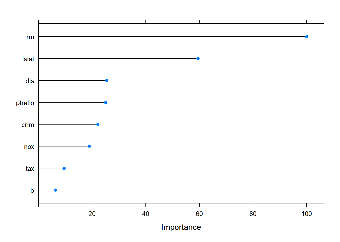
# the plot of performance of model
df_mars <- data.frame(predicted = as.numeric(mars_pred), observed = testset$medv,
                     residual = as.numeric(testset$medv - mars_pred))

ggplot(df_mars, aes(x = predicted, y = observed)) +
  geom_point() +
  geom_abline(intercept = 0, slope = 1, colour = "blue") +
  ggtitle("MARS Predicted VS Observed")
ggplot(df_mars, aes(x = predicted, y = residual)) +
  geom_point() +
  geom_hline(yintercept = 0, colour = "blue") +
  ggtitle("MARS Predicted VS Residual")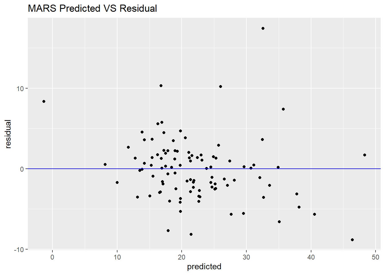
Support Vector Machines
SVM are a powerful, flexible model.
There are some kernel functions that can be used to generalize the regression model and encompass nonlinear functions of the predictors.
The cost parameter is the main tool for adjusting the complexity of the model.
When the cost is large, the model becomes very flexible; when the cost is small, the model more likely to under-fit.
Since the predictors enter into the model as the sum of cross products, differences in the predictor scales can affect the model.
Therefore, we should centering and scaling the predictors prior to building an SVM model.
#####################################
### support vector machines
# need preprocess to data
set.seed(1234)
svm_radial_model <- train(medv ~ .,
                         data = trainset,
                         method = "svmRadial",
                         preProc = c("center", "scale"),
                         tuneLength = 14,
                         trControl = trainControl(method= "cv"))
svm_radial_model
## Support Vector Machines with Radial Basis Function Kernel
##
## 407 samples
## 13 predictor
##
## Pre-processing: centered (13), scaled (13)
## Resampling: Cross-Validated (10 fold)
## Summary of sample sizes: 366, 367, 365, 366, 366, 366, ...
## Resampling results across tuning parameters:
##
## C RMSE Rsquared MAE
## 0.25 4.748972 0.7794030 2.862857
## 0.50 4.183735 0.8188077 2.572342
## 1.00 3.845921 0.8418180 2.430202
## 2.00 3.598909 0.8582325 2.315648
## 4.00 3.412456 0.8721668 2.264396
## 8.00 3.360851 0.8756835 2.259172
## 16.00 3.301545 0.8806566 2.215076
## 32.00 3.339069 0.8782759 2.257679
## 64.00 3.418751 0.8723520 2.335112
## 128.00 3.623009 0.8593733 2.471478
## 256.00 3.710921 0.8522589 2.551034
## 512.00 3.750931 0.8480772 2.598195
## 1024.00 3.841863 0.8394062 2.655697
## 2048.00 4.009463 0.8270005 2.762089
##
## Tuning parameter 'sigma' was held constant at a value of 0.09990706
## RMSE was used to select the optimal model using the smallest value.
## The final values used for the model were sigma = 0.09990706 and C = 16.svm_radial_pred <- predict(svm_radial_model, testset)
postResample(pred = svm_radial_pred, obs = testset$medv)## RMSE Rsquared MAE
## 3.0314516 0.8553794 2.1361834update(plot(svm_radial_model, scales = list(x = list(log = 2))),
main = "The Cross-Validation Profiles for SVM Radial Model") 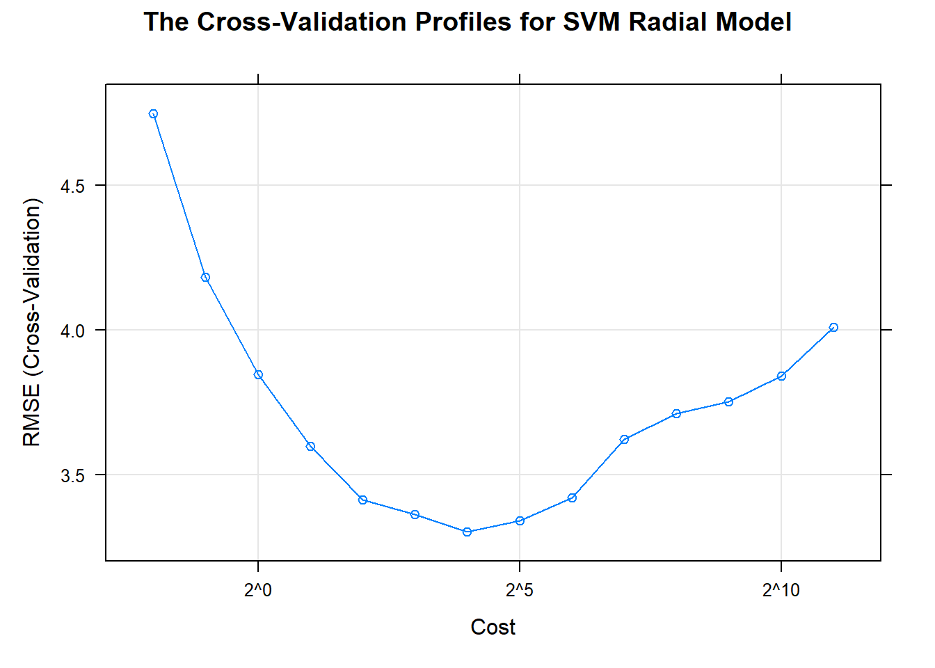
K-Nearest Neighbors
The KNN approach simply predicts a new sample using the K-closest samples from the training set.
The basic KNN method depends on how the user defines distance between samples, so the scale of the predictors can have a dramatic influence on the distances among samples.
To avoid this potential bias, we recommend that all predictors be centered and scaled prior to performing KNN.
In addition to the scaling, if there are some missing predictors values, then the distances between predictors are not be computed, we could excluded the missing values or impute the missing data use some methods.
The KNN method can have poor predictive performance when there are some irrelevant or noisy predictors, which can cause similar samples to be driven away from each other in the predictor space.
Hence, removing irrelevant, noise-laden predictors is a key-processing step for KNN.
#####################################
### k-nearest neighbors
# need preprocess to data
set.seed(1234)
knn_model <- train(trainset[, 1:13], trainset[, 14],
                  method = "knn",
                  preProc = c("center", "scale"),
                  tuneGrid = data.frame(k = 1:20),
                  trControl = trainControl(method= "cv"))
knn_model
## k-Nearest Neighbors
##
## 407 samples
## 13 predictor
##
## Pre-processing: centered (12), scaled (12), ignore (1)
## Resampling: Cross-Validated (10 fold)
## Summary of sample sizes: 366, 367, 365, 366, 366, 366, ...
## Resampling results across tuning parameters:
##
## k RMSE Rsquared MAE
## 1 4.529964 0.7902339 3.010800
## 2 3.735091 0.8523374 2.510353
## 3 3.763624 0.8504123 2.570824
## 4 3.900365 0.8418691 2.639117
## 5 4.032804 0.8348617 2.673419
## 6 4.057364 0.8328166 2.697384
## 7 4.186697 0.8243871 2.779620
## 8 4.266893 0.8173155 2.817948
## 9 4.359553 0.8096479 2.904049
## 10 4.413786 0.8035681 2.936118
## 11 4.430084 0.8033026 2.941730
## 12 4.476100 0.8027364 2.968149
## 13 4.532325 0.7984077 3.036164
## 14 4.548150 0.7968115 3.045181
## 15 4.575902 0.7947727 3.065290
## 16 4.612420 0.7912686 3.096591
## 17 4.649984 0.7878617 3.125036
## 18 4.705139 0.7842849 3.159568
## 19 4.766942 0.7794370 3.203215
## 20 4.795894 0.7769760 3.205589
##
## RMSE was used to select the optimal model using the smallest value.
## The final value used for the model was k = 2.knn_pred <- predict(knn_model, testset[, 1:13])
postResample(pred = knn_pred, obs = testset$medv)## RMSE Rsquared MAE
## 3.4077526 0.8189149 2.4414141update(plot(knn_model), main = "The Cross-Validation Profiles for KNN Model")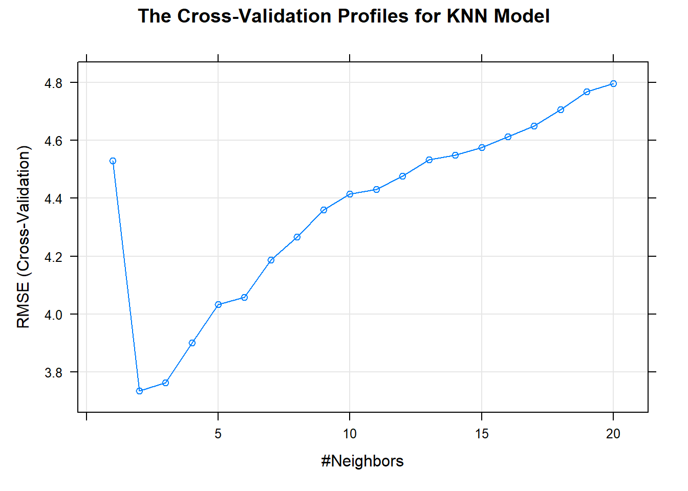
Referenced:
Applied Predictive Modeling
Just record, this article was posted at linkedin, and have 362 views to November 2021.