Classification Model Series I : Do Some Classification Models In R By Iris Data Set
2016-02-19
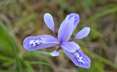
This famous (Fisher’s or Anderson’s) iris data set gives the measurements in centimeters of the variables sepal length and width and petal length and width, respectively, for 50 flowers from each of 3 species of iris. The species are Iris setosa, versicolor, and virginica.
###################################################
### use iris dataset to test classify models
###################################################

# load the data set
data(iris)

#########################
# explore the data set
#########################

head(iris)
## Sepal.Length Sepal.Width Petal.Length Petal.Width Species
## 1 5.1 3.5 1.4 0.2 setosa
## 2 4.9 3.0 1.4 0.2 setosa
## 3 4.7 3.2 1.3 0.2 setosa
## 4 4.6 3.1 1.5 0.2 setosa
## 5 5.0 3.6 1.4 0.2 setosa
## 6 5.4 3.9 1.7 0.4 setosastr(iris)## 'data.frame': 150 obs. of 5 variables:
## $ Sepal.Length: num 5.1 4.9 4.7 4.6 5 5.4 4.6 5 4.4 4.9 ...
## $ Sepal.Width : num 3.5 3 3.2 3.1 3.6 3.9 3.4 3.4 2.9 3.1 ...
## $ Petal.Length: num 1.4 1.4 1.3 1.5 1.4 1.7 1.4 1.5 1.4 1.5 ...
## $ Petal.Width : num 0.2 0.2 0.2 0.2 0.2 0.4 0.3 0.2 0.2 0.1 ...
## $ Species : Factor w/ 3 levels "setosa","versicolor",..: 1 1 1 1 1 1 1 1 1 1 ...summary(iris)## Sepal.Length Sepal.Width Petal.Length Petal.Width Species
## Min. :4.300 Min. :2.000 Min. :1.000 Min. :0.100 setosa :50
## 1st Qu.:5.100 1st Qu.:2.800 1st Qu.:1.600 1st Qu.:0.300 versicolor:50
## Median :5.800 Median :3.000 Median :4.350 Median :1.300 virginica :50
## Mean :5.843 Mean :3.057 Mean :3.758 Mean :1.199
## 3rd Qu.:6.400 3rd Qu.:3.300 3rd Qu.:5.100 3rd Qu.:1.800
## Max. :7.900 Max. :4.400 Max. :6.900 Max. :2.500Let us see some relationships between variables in the iris data set.
#  visualizing relationships between variables
library(ggplot2)
ggplot(iris, aes(x = Sepal.Length, y = Sepal.Width, col = Species, shape = Species)) +
  geom_point()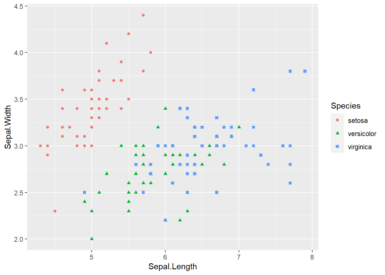
ggplot(iris, aes(x = Sepal.Length, y = Petal.Length, col = Species, shape = Species)) +
  geom_point()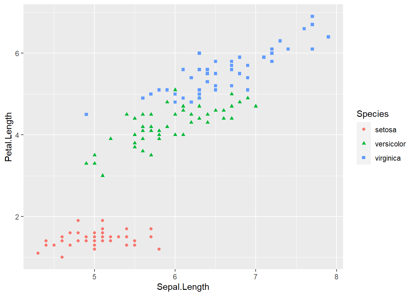
ggplot(iris, aes(x = Sepal.Length, y = Petal.Width, col = Species, shape = Species)) +
  geom_point()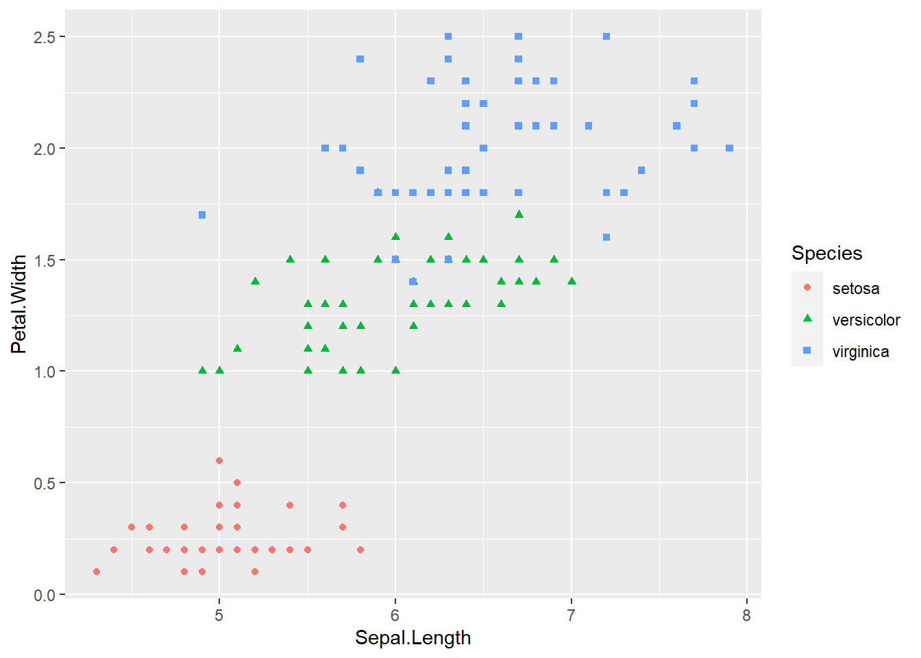
ggplot(iris, aes(x = Sepal.Width, y = Petal.Length, col = Species, shape = Species)) +
  geom_point()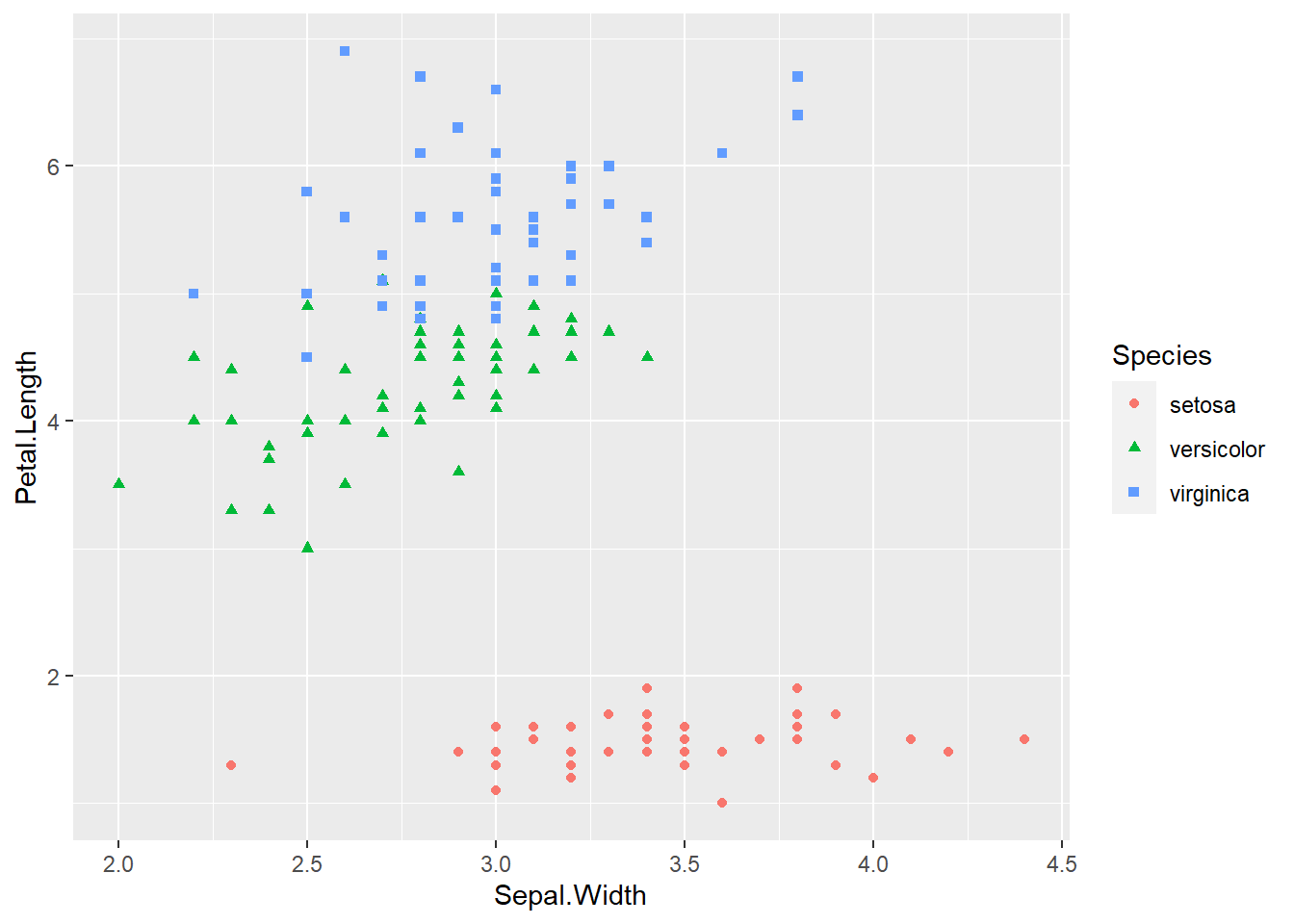
ggplot(iris, aes(x = Sepal.Width, y = Petal.Width, col = Species, shape = Species)) +
  geom_point()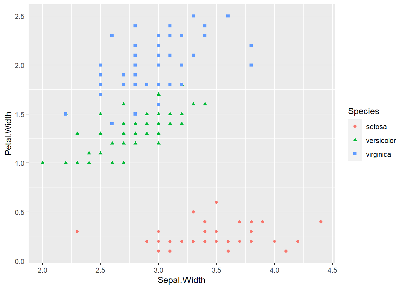
ggplot(iris, aes(x = Petal.Width, y = Petal.Length, col = Species, shape = Species)) +
geom_point()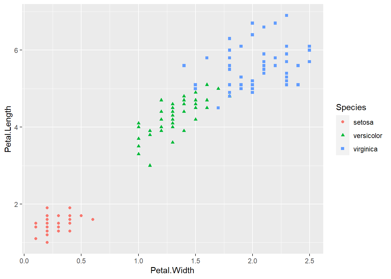 The species of setosa is easy identify by petal width or petal length, the other species are somewhat difficult to classify.
Then we split iris data set to train-set and test-set.
#########################################
##  split the data set to train and test
#########################################

n <- length(iris[,1])
index1 <- 1 : n
# divide to 5 part of data
index2 <- rep(1 : 5, ceiling(n / 5))[1 : n]
set.seed(100)
# melt the order of the data
index2 <- sample(index2, n)
# get the one part of the data
m <- index1[index2 == 1]
trainset <- iris[-m, ]
testset <- iris[m, ]
str(trainset)
## 'data.frame': 120 obs. of 5 variables:
## $ Sepal.Length: num 5.1 4.9 4.7 4.6 5 5.4 4.6 5 4.4 4.9 ...
## $ Sepal.Width : num 3.5 3 3.2 3.1 3.6 3.9 3.4 3.4 2.9 3.1 ...
## $ Petal.Length: num 1.4 1.4 1.3 1.5 1.4 1.7 1.4 1.5 1.4 1.5 ...
## $ Petal.Width : num 0.2 0.2 0.2 0.2 0.2 0.4 0.3 0.2 0.2 0.1 ...
## $ Species : Factor w/ 3 levels "setosa","versicolor",..: 1 1 1 1 1 1 1 1 1 1 ...Let us try to do some classification models.
Logistic regression is mainly for 2 response classes, and for linear decision boundaries.Of course, we could also classify the species of setosa first, then use logic regression to classify the other species, but we did not try it in here.
Discriminant analysis is popular for multiple-class classification.Here, we assume the decision boundary is linear, so we use linear discriminant analysis model.
#####################################
## try kinds of classify models
#####################################

## linear discriminant analysis
library(MASS)
lda_model <- lda(Species ~ ., data = trainset)
lda_model
## Call:
## lda(Species ~ ., data = trainset)
##
## Prior probabilities of groups:
## setosa versicolor virginica
## 0.3333333 0.3333333 0.3333333
##
## Group means:
## Sepal.Length Sepal.Width Petal.Length Petal.Width
## setosa 4.9700 3.3975 1.4625 0.2425
## versicolor 5.9075 2.7525 4.2450 1.3150
## virginica 6.6300 2.9975 5.5900 2.0400
##
## Coefficients of linear discriminants:
## LD1 LD2
## Sepal.Length 0.6090357 0.06544054
## Sepal.Width 1.4196508 2.20984856
## Petal.Length -2.0519675 -0.91661473
## Petal.Width -2.8551780 2.70280342
##
## Proportion of trace:
## LD1 LD2
## 0.9896 0.0104plot(lda_model)
lda_pred <- predict(lda_model, testset)Let us see the confusion matrix and accurate from linear discriminant analysis model.
table(lda_pred$class, testset$Species)##
## setosa versicolor virginica
## setosa 10 0 0
## versicolor 0 10 1
## virginica 0 0 9mean(lda_pred$class == testset$Species)## [1] 0.9666667K-nearest neighbor model is mainly for complicated decision boundary, and for few features.If there are much many features, this model will dive into the curse of dimension.
In this model, the scale of the variables matters, because this classifier predicts the class of a given test observation by identifying distance, so to standardize the data is a good way.
## k-nearest neighbor
library(class)
train_x <- as.matrix(trainset[, 1:4])
test_x <- as.matrix(testset[, 1:4])
train_y <- trainset[, 5]

set.seed(1)
knn_pred <- knn(train_x, test_x, train_y, k = 1)

table(knn_pred, testset$Species)
##
## knn_pred setosa versicolor virginica
## setosa 10 0 0
## versicolor 0 10 2
## virginica 0 0 8mean(knn_pred == testset$Species)## [1] 0.9333333Decision tree is a classic model. It is simple and easy to explain to people.However, trees generally do not have high accuracy.
## decision tree
library(tree)
## Registered S3 method overwritten by 'tree':
## method from
## print.tree clitree_model <- tree(Species ~ ., trainset)
summary(tree_model)##
## Classification tree:
## tree(formula = Species ~ ., data = trainset)
## Variables actually used in tree construction:
## [1] "Petal.Length" "Petal.Width" "Sepal.Length"
## Number of terminal nodes: 5
## Residual mean deviance: 0.1813 = 20.85 / 115
## Misclassification error rate: 0.03333 = 4 / 120Decision tree can be displayed graphically.
plot(tree_model)
text(tree_model, pretty = 0)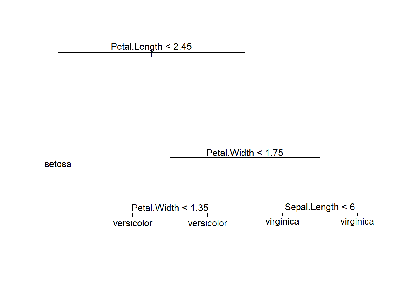 The confusion matrix and accuracy from decision tree model.
tree_pred <- predict(tree_model, testset, type = "class")

table(tree_pred, testset$Species)
##
## tree_pred setosa versicolor virginica
## setosa 10 0 0
## versicolor 0 10 2
## virginica 0 0 8mean(tree_pred == testset$Species)## [1] 0.9333333By aggregating many decision trees, using models like bagging, random forests, and boosting, the accuracy of tree can be substantially improved.
## bagging
library(randomForest)
## randomForest 4.6-14## Type rfNews() to see new features/changes/bug fixes.##
## 载入程辑包:'randomForest'## The following object is masked from 'package:ggplot2':
##
## marginbag_model <- randomForest(Species ~ ., data = trainset, mtry = 4,
importance = TRUE)
bag_model##
## Call:
## randomForest(formula = Species ~ ., data = trainset, mtry = 4, importance = TRUE)
## Type of random forest: classification
## Number of trees: 500
## No. of variables tried at each split: 4
##
## OOB estimate of error rate: 4.17%
## Confusion matrix:
## setosa versicolor virginica class.error
## setosa 40 0 0 0.000
## versicolor 0 37 3 0.075
## virginica 0 2 38 0.050bag_pred <- predict(bag_model, newdata = testset)
plot(bag_pred, testset$Species)
table(bag_pred, testset$Species)##
## bag_pred setosa versicolor virginica
## setosa 10 0 0
## versicolor 0 10 2
## virginica 0 0 8mean(bag_pred == testset$Species)## [1] 0.9333333The main difference between bagging and random forests is the choice of predictor subset size.
##  random forestlibrary(randomForest)
rf_model <- randomForest(Species ~ ., data = trainset,
                          importance = TRUE)
rf_model
##
## Call:
## randomForest(formula = Species ~ ., data = trainset, importance = TRUE)
## Type of random forest: classification
## Number of trees: 500
## No. of variables tried at each split: 2
##
## OOB estimate of error rate: 5%
## Confusion matrix:
## setosa versicolor virginica class.error
## setosa 40 0 0 0.000
## versicolor 0 37 3 0.075
## virginica 0 3 37 0.075Random forest could also supply us the importance of variables.
rf_pred <- predict(rf_model, newdata = testset)
plot(rf_pred, testset$Species)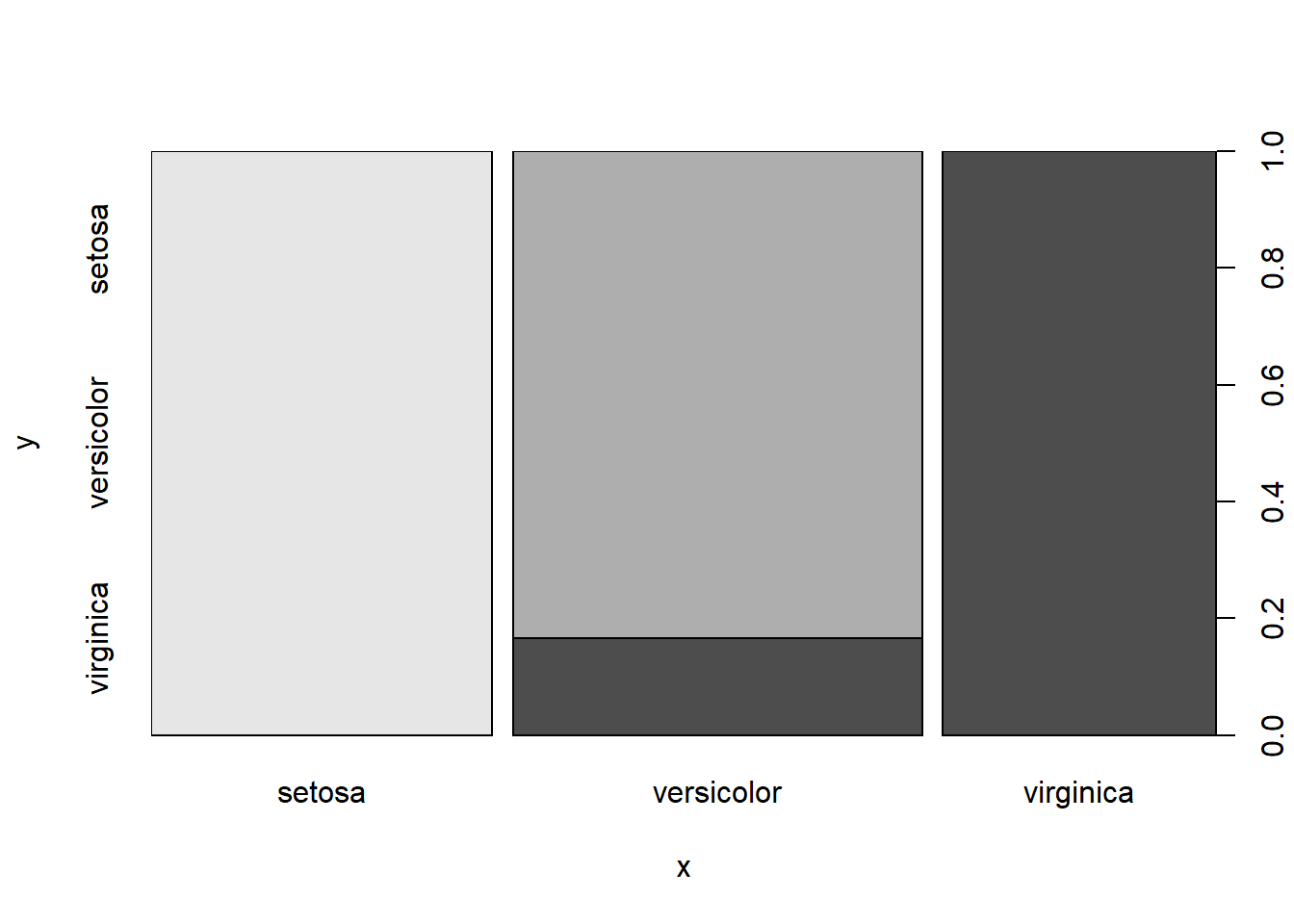
importance(rf_model)## setosa versicolor virginica MeanDecreaseAccuracy MeanDecreaseGini
## Sepal.Length 7.613543 6.818930 9.557335 11.838471 9.273543
## Sepal.Width 5.531353 2.260127 3.547368 5.997058 2.151328
## Petal.Length 23.581406 29.663793 26.582862 33.405993 33.149589
## Petal.Width 20.999556 27.430154 34.330308 33.420164 34.668673varImpPlot(rf_model)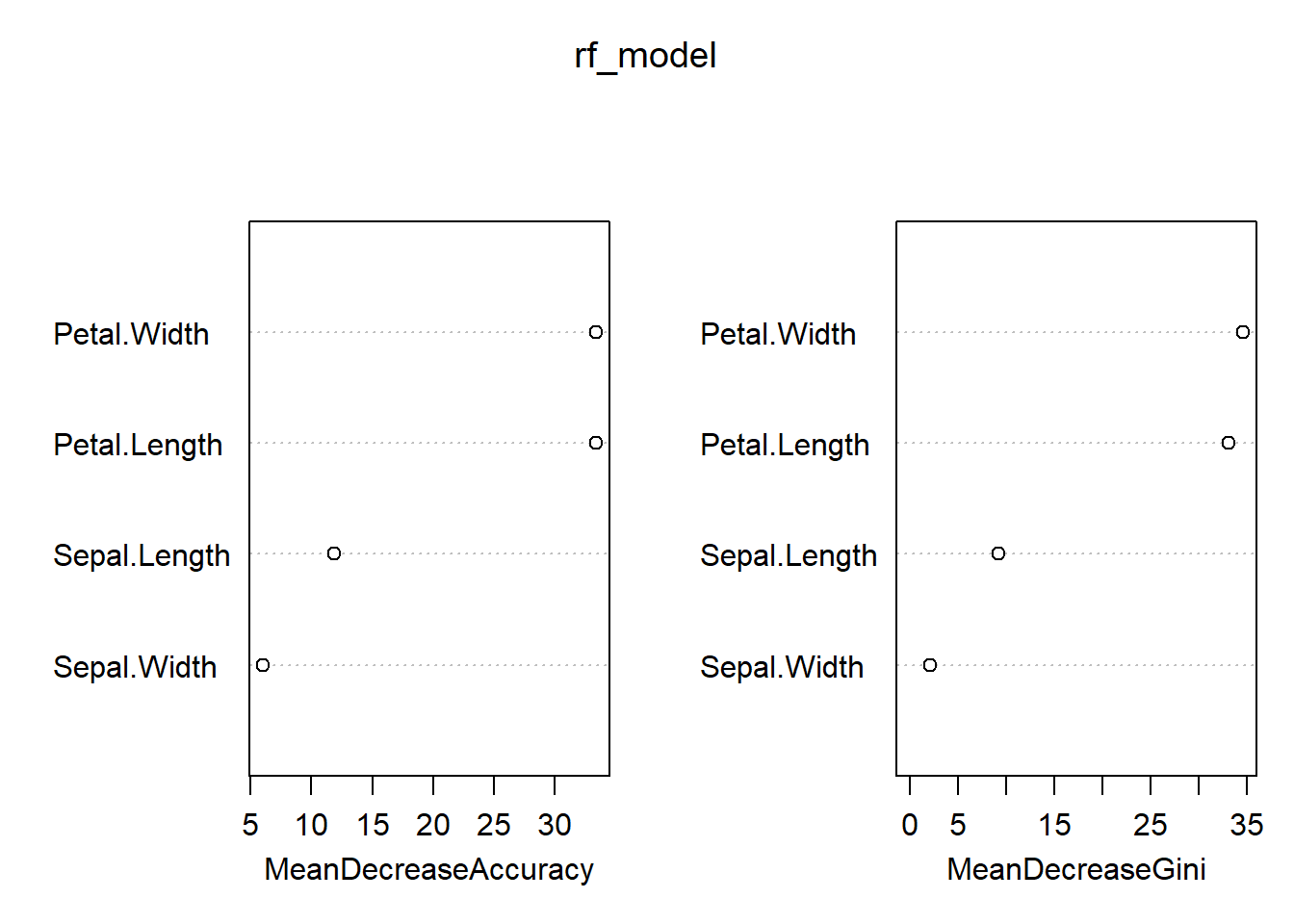
table(rf_pred, testset$Species)##
## rf_pred setosa versicolor virginica
## setosa 10 0 0
## versicolor 0 10 2
## virginica 0 0 8mean(rf_pred == testset$Species)## [1] 0.9333333In boosting, because the growth of a particular tree takes into account the other trees that have already been grown, smaller trees are typically sufficient.
## boosting
library(gbm)
## Loaded gbm 2.1.8boost_model <- gbm(Species ~ ., data = trainset)## Distribution not specified, assuming multinomial ...## Warning: Setting `distribution = "multinomial"` is ill-advised as it is currently broken. It exists
## only for backwards compatibility. Use at your own risk.summary(boost_model)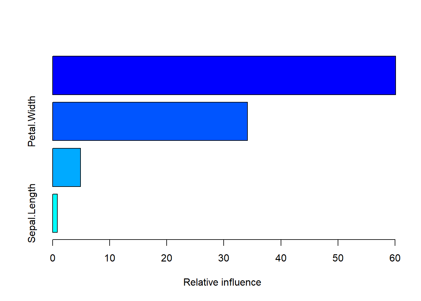
##                       var    rel.inf
## Petal.Length Petal.Length 60.1021627
## Petal.Width   Petal.Width 34.1425780
## Sepal.Width   Sepal.Width  4.9146578
## Sepal.Length Sepal.Length  0.8406015
boost_pred <- predict(boost_model, newdata = testset, n.trees = 100,
type = "response")
temp = data.frame(boost_pred[, , 1])
temp2 = apply(temp, 1, which.max)
boost_pred2 <- names(temp)[temp2]
table(boost_pred2, testset$Species)##
## boost_pred2 setosa versicolor virginica
## setosa 10 0 0
## versicolor 0 10 2
## virginica 0 0 8mean(boost_pred2 == testset$Species)## [1] 0.9333333Support vector machine model:
##  support vector machine
library(e1071)
svm_model <- svm(Species ~ ., data = trainset,
                 kernel = "linear", scale = FALSE)
summary(svm_model)
##
## Call:
## svm(formula = Species ~ ., data = trainset, kernel = "linear", scale = FALSE)
##
##
## Parameters:
## SVM-Type: C-classification
## SVM-Kernel: linear
## cost: 1
##
## Number of Support Vectors: 23
##
## ( 3 11 9 )
##
##
## Number of Classes: 3
##
## Levels:
## setosa versicolor virginicasvm_pred <- predict(svm_model, testset)
table(svm_pred, testset$Species)##
## svm_pred setosa versicolor virginica
## setosa 10 0 0
## versicolor 0 10 0
## virginica 0 0 10mean(svm_pred == testset$Species)## [1] 1Naive bayes model:
## naive bayes
library(e1071)
bayes_model <- naiveBayes(trainset[, 1:4], trainset$Species)
summary(bayes_model)
## Length Class Mode
## apriori 3 table numeric
## tables 4 -none- list
## levels 3 -none- character
## isnumeric 4 -none- logical
## call 3 -none- callbayes_pred <- predict(bayes_model, testset[, 1:4], type = "class")
table(bayes_pred, testset$Species)##
## bayes_pred setosa versicolor virginica
## setosa 10 0 0
## versicolor 0 9 2
## virginica 0 1 8mean(bayes_pred == testset$Species)## [1] 0.9Artificial neural networks model:
## artificial neural networks
library(nnet)
ann_model <- nnet(Species ~ ., data = trainset, size = 3)
## # weights: 27
## initial value 131.269030
## iter 10 value 55.781204
## iter 20 value 55.461173
## iter 30 value 55.453487
## iter 40 value 55.414230
## iter 50 value 48.507540
## iter 60 value 12.162402
## iter 70 value 4.001708
## iter 80 value 1.190122
## iter 90 value 0.029758
## iter 100 value 0.000278
## final value 0.000278
## stopped after 100 iterationsann_pred <- predict(ann_model, newdata = testset, type = "class")
table(ann_pred, testset$Species)##
## ann_pred setosa versicolor virginica
## setosa 10 0 0
## versicolor 0 10 3
## virginica 0 0 7mean(ann_pred == testset$Species)## [1] 0.9There are three models achieved highest correct rate 0.9666667.
They are linear discriminant analysis, support vector machine and artificial neural net.
Referenced books:
Machine Learning with R
Applied Predictive Modeling
An Introduction to Statistical Learning with Applications in R
Just record, this article was posted at linkedin, and have 238 views to November 2021.